ContentsNews
Metadynminer and Metadynminer3D paper out in R Journal: Videos from Metadynminer Plumed Masterclass (February 2022) are available at Youtube (thanks to Plumed!!!): Video from Metadynminer webinar (31 May 2019) is available at Youtube (thanks to ELIXIR Slovenia!!!): Metadynminer3d was published. See comparison of accuracy of Introductionmetadynminer is R packages for reading, analysis and visualization of metadynamics HILLS files produced by Plumed [1]. It reads HILLS files from Plumed, calculates free energy surfaces by fast Bias Sum algorithm [2], finds minima and analyses transition paths by Nudged Elastic Band method [3].SourceUsageInstalationTo install R go to https://www.r-project.org/. It is available for a variety of UNIX platforms, Windows and MacOS, as well as for cloud environment. You can also use some fancy environments such as https://www.rstudio.com/.
Command lines in R enviroment start with Install a stable version of metadynminer from CRAN by starting the R environment and typing: > install.packages("metadynminer")If you want to install a development version of the package from github, you need to install devtools: > install.packages("devtools") > library(devtools) > devtools::install_github("spiwokv/metadynminer") Next, invoke metadynminer:
> library(metadynminer)
Help can be obtained by the function help() with the name of the function
as the argument, or by a question mark followed by the name of the function:
> help(read.hills)
> ?read.hills
Reading HILLS filesA Plumed HILLS file can be loaded by typing:> hillsf<-read.hills("HILLS") 2D HILLS file readThis assumes that the hills file is in the working directory. If not you can specify the path (e.g. "../mymetadynamics/HILLS"). Alternatively you can check
path by typing:
> getwd()
[1] "/home/yourlogin/somedirectory"
and you can change working directory by typing: > setwd("/home/yourlogin/directory")(may be useful in MS Windows). Hills file can be also loaded from a web site by using its URL: > hillsf<-read.hills("http://www.metadynamics.cz/metadynminer/data/HILLS2d") 2D HILLS file read metadynminer accepts only hills files with one or two collective variables.
If some of collective variables is periodic (usually a torsion) it is necessary to specify
this fact at the moment of loading of hills file by parameter > hillsf<-read.hills("HILLS", per=c(TRUE, TRUE)) 2D HILLS file readCollective variables are not periodic by default.
Period of a periodic collective variable is by default set to -π to +π. It can be
changed by setting parameters > hillsf<-read.hills("HILLS", per=c(TRUE, TRUE), pcv1=c(0,2*pi)) 2D HILLS file readmetadynminer contains two preloaded data set (two hills files), one for Alanine Dipeptide in water with Ramachandran angles φ and ψ as collective variables (called acealanme)
and one for the same system with only one collective variable φ (called acealanme1d).
Metadynamics simulations are very often split into multiple runs with
However, a user can load hills from restarted simulations without this option. First, wrong time values
do not affect calculations of free energy surfaces. Second, the option
The package metadynminer provides > acealanme 2D hills file HILLS2d with 30000 lines > summary(acealanme) 2D hills file HILLS2d with 30000 lines The CV1 ranges from -3.141309 to 3.14159 The CV2 ranges from -3.141321 to 3.141371Hills file objects can be concatenated by addition ( +) operation:
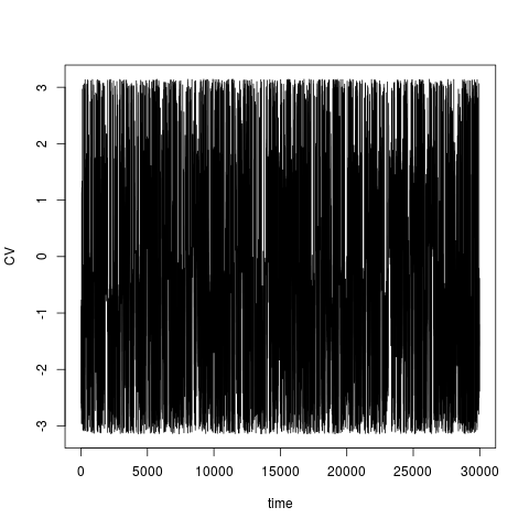
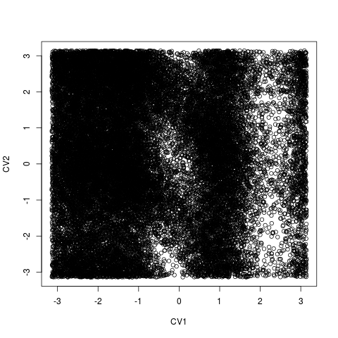
> acealanme+acealanme
2D hills file HILLS2d with 60000 lines
metadynminer provides plot function for its objects. Hills file with one collective variable will be pllotted as the evolution of the collective variable.
> plot(acealanme1d)
Hills file with two collective variables will be plotted as collective variable 1 vs. collective variable 2.
> plot(acealanme)
In a plot you can modify labels of axes (
It is possible to use
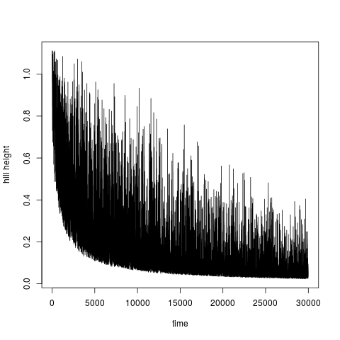
Beside the function In well tempered metadynamics [4] it is useful to see evolution of heights of hills. This can be ploted by typing:
> plotheights(acealanme)
It is again possible to use Calculation of free energy surfaceFree energy surface is calculated by summing hills using functionfes:
> tfes<-fes(hillsf)Summing hills is much less expensive than a metadynamics simulation, nevertheless, it can be a slow process if number of hills exceeds 10,000. We developed a Bias Sum algorithm [2] to accelerate this calculation. Instead of evaluation exp(-||s-St||2/2σ2) for every hill it calculates a single Gaussian hill and relocates it. This function is not available for simulations with variable hill widths. As an alternative it is possible to calculate free energy surface by conventional way (function fes2). This function works with variable hill widths:
> tfes<-fes2(hillsf)Hills can be summed for whole simulation (default) or for selected hills. The range can be controlled by imin and imax. These are indexes of first and last hill to be summed.
> tfes<-fes(hillsf, imin=5000, imax=10000)By default the free energy surface is calculated for 256 (1D) or 256x256 (2D) grid points. This can be changed by npoints option.
Two free energy surfaces can be added and subtracted: > tfes 2D free energy surface with 256 x 256 points, maximum -23.96706 and minimum -97.32465 > tfes+tfes 2D free energy surface with 256 x 256 points, maximum -47.93411 and minimum -194.6493 > tfes-tfes Warning: FES obtained by subtraction of two FESes will inherit hills only from the first FES 2D free energy surface with 256 x 256 points, maximum 0 and minimum 0It is possible to add or subtract a constant. Free energy surface can be also multiplied or divided by a constant: > tfes/4.184 Warning: division of FES will divide the FES but not hill heights 2D free energy surface with 256 x 256 points, maximum -5.728264 and minimum -23.26115It is possible to calculate minimum and maximum of free energy surface by functions min and
max, respectively. This can be used, for example, to convert a free energy surface so that
the global minimum is equal to zero:
> tfes-min(tfes)
2D free energy surface with 256 x 256 points, maximum 73.35759 and minimum 0
The function summary function gives the same output as print for free energy
surface object:
tfes
2D free energy surface with 256 x 256 points, maximum -23.96706 and minimum -97.32465
summary(tfes)
2D free energy surface with 256 x 256 points, maximum -23.96706 and minimum -97.32465
Plotting of free energy surfaceFree energy surface can be plotted by functionplot. This function behaves differently depending
on dimensionality of the free energy surface. For 1D surface it plots the profile:
> tfes<-fes(acealanme1d) > plot(tfes) 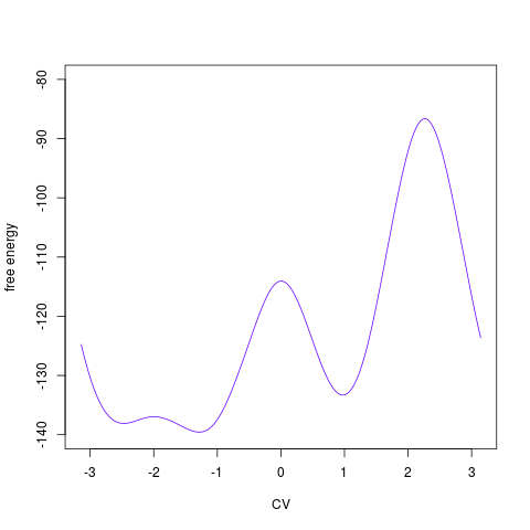
For 2D surface it plots the free energy surface by R function > tfes<-fes(acealanme) > plot(tfes) 
The type of a 2D plot can be controlled by
Similarly to hills file you can modify labels of axes (
For 1D surface you can modify the color of line by
For 2D surface it is possible to chose whether it is ploted as a heatmap (R function > tfes<-fes(acealanme) > tfes<-tfes-min(tfes) > plot(tfes, zlim=c(0,200), nlevels=20) 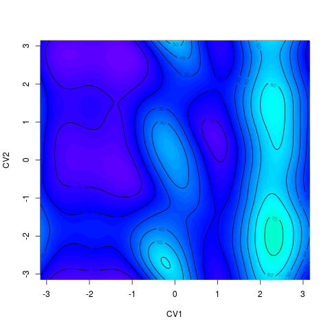
You can also implicitly specify contour values explicitely by > plot(tfes, zlim=c(0,200), levels=1:20*10)Here 1:20 returns 1, 2 ... 20 and 1:20*10 return 10, 20 ... 200.
Color scale can be printed by option > tfes<-fes(acealanme) > plot(tfes, colscale=TRUE) 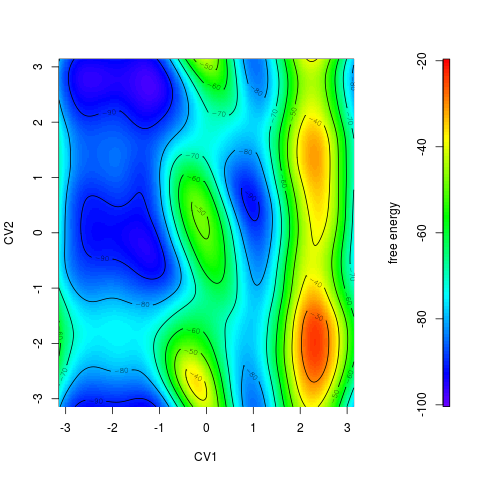
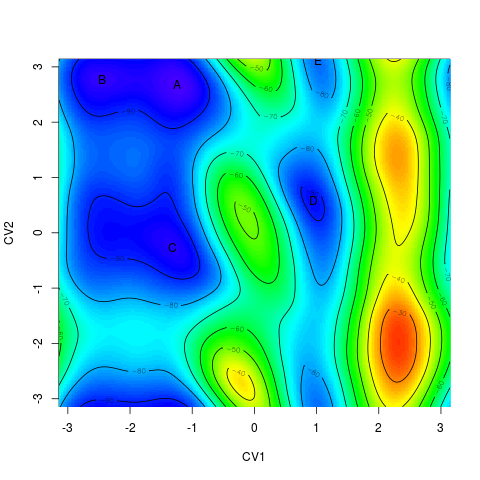
Identification of minimaFree energy minima corresponds to stable or metastable states of the studied system. You can use functionfesminima to automatically locate free energy minima
on the free energy surface:
> tfes<-fes(acealanme)
> minima<-fesminima(tfes)
This function divides the free energy surface into 8 (1D) or 8x8 (2D) equivalent bins. For each bin it finds its energy minimum. Next, it checks whether these minima are local minima of the whole surface. These minima are collected, sorted and labeled by alphabet letters. The number of bins can be modified by parameter nbins.
Functions > minima $minima letter CV1bin CV2bin CV1 CV2 free_energy 1 A 78 237 -1.2443171 2.6734337 -97.32465 2 B 29 241 -2.4516743 2.7719935 -95.77144 3 C 75 118 -1.3182369 -0.2587194 -94.66432 4 D 167 152 0.9486378 0.5790386 -91.86909 5 E 170 255 1.0225576 3.1169527 -84.57032 > summary(minima) [1] 6 letter CV1bin CV2bin CV1 CV2 free_energy relative_pop 1 A 78 237 -1.2443171 2.6734337 -97.32465 8.837680e+16 2 B 29 241 -2.4516743 2.7719935 -95.77144 4.741231e+16 3 C 75 118 -1.3182369 -0.2587194 -94.66432 3.041705e+16 4 D 167 152 0.9486378 0.5790386 -91.86909 9.917603e+15 5 E 170 255 1.0225576 3.1169527 -84.57032 5.315355e+14 pop 1 50.0278223 2 26.8388849 3 17.2183058 4 5.6140985 5 0.3008885The function summary calculate equilibrium populations of each minimum in percent.
Keep in mind that these values were calculated from free energies of minima points, not by
integrating populations of each free energy minimum basin. These values are dependent on
temperature and energy units. By default these are set to temp=300 and
eunit="kJ/mol". The parameter eunit can be set to "kJ/mol"
or "kcal/mol".
Sometimes it is useful to add some point in the space of collective variables to the list of automatically identified minima. This can be done by making a "fake" minimum and adding it to the list: > minima<-fesminima(tfes)+oneminimum(tfes, cv1=0, cv2=0) > minima $minima letter CV1bin CV2bin CV1 CV2 free_energy 1 A 78 237 -1.2443171 2.6734337 -97.32465 2 B 29 241 -2.4516743 2.7719935 -95.77144 3 C 75 118 -1.3182369 -0.2587194 -94.66432 4 D 167 152 0.9486378 0.5790386 -91.86909 5 E 170 255 1.0225576 3.1169527 -84.57032 6 F 129 129 0.0000000 0.0000000 -49.33291This will create the same set of minima with the additional one placed in the point {0,0}.
The function
> plot(minima)
Color of labels can be controlled by Calculation of free energy profilesImagine metadynamics of a system with two energy minima, one (A) at 0 kJ/mol and the second (B) at 10 kJ/mol, separated by a transition state (TS) at 30 kJ/mol. We want to estimate the free energy difference between B and A. At the begining of metadynamics it is estimated as zero, because there is no bias potential. Metadynamics starting from B would flood this minimum after some time. At this point the free energy estimate is -20 kJ/mol. Next, the system jumps to A. After flooding A the free energy estimate reaches the correct value of 10 kJ/mol. After this point the system can freely jump from A to B and B to A because both minima are flooded and the free energy surface is flattened. This leads to oscillation of free energy difference around the correct value of 10 kJ/mol. It is therefore useful to examine the evolution of free energy difference during the simulation. Convergence of these values indicate (but do not fully proof) that the estimated free energy difference is accurate.
This can be evaluated by function > tfes<-fes(acealanme) > minima<-fesminima(tfes) > prof<-feprof(minima)This function calculates evolution of free energy differences between each minimum and the global minimum (global at the end of simulation).Free energy of the global minimum is always zero.
Similarly to functions
It is possible to use functions > prof 30001 2D minima > summary(prof) letter CV1bin CV2bin CV1 CV2 free_energy min diff max diff 1 A 78 237 -1.2443171 2.6734337 -97.32465 0.0000000 0.000000 2 B 29 241 -2.4516743 2.7719935 -95.77144 -2.0561128 3.731685 3 C 75 118 -1.3182369 -0.2587194 -94.66432 0.3887439 12.213005 4 D 167 152 0.9486378 0.5790386 -91.86909 0.7606614 21.746684 5 E 170 255 1.0225576 3.1169527 -84.57032 0.8638223 21.746684 tail 1 0.000000 2 1.637328 3 2.670321 4 5.497148 5 12.875954The function summary prints minimal and maximal free energy difference
for time range specified by imind and imaxd. For example,
it is possible to calculate the free energy surface from all hills and evaluate
convergence of the free energy difference in last 10,000 hills:
> tfes<-fes(acealanme) > minima<-fesminima(tfes) > prof<-feprof(minima) > summary(prof, imind=20000, imaxd=30000) letter CV1bin CV2bin CV1 CV2 free_energy min diff max diff 1 A 78 237 -1.2443171 2.6734337 -97.32465 0.0000000 0.000000 2 B 29 241 -2.4516743 2.7719935 -95.77144 0.4399352 1.700877 3 C 75 118 -1.3182369 -0.2587194 -94.66432 1.1614741 3.229472 4 D 167 152 0.9486378 0.5790386 -91.86909 4.4346671 5.967618 5 E 170 255 1.0225576 3.1169527 -84.57032 11.0699007 13.173305 tail 1 0.000000 2 1.637328 3 2.670321 4 5.497148 5 12.875954This shows that the free energy of B (realtive to A) was 0.4399352-1.700877 and value at the end of simulation (in imaxd) was 1.637328 kJ/mol.
Profiles can be plotted using
> plot(prof)
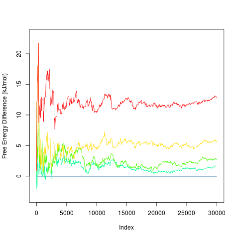
By default it plots profiles for all free energy minima. It is possible to specify minima to be
plotted by Removing one collective variableSometimes it may be useful to get rid of one collective variable by calculating a 1D free energy surface from a 2D one. It is not possible to do this simply by ignoring on collective variable in the hills summing process. Instead, it is necessary to convert 2D free energy surface into probabilities (as exp(-F/kT)), integrate probabilities along one collective variable and convert probabilities back to free energies (as -kTlog(P)). This can be done by functionfes2d21d:
> tfes1<-fes2d21d(acealanme, remdim=2) > plot(tfes1) 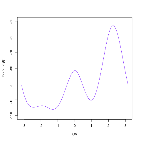
The process depends on temperature of simulation and energy units. It is therefore possible to
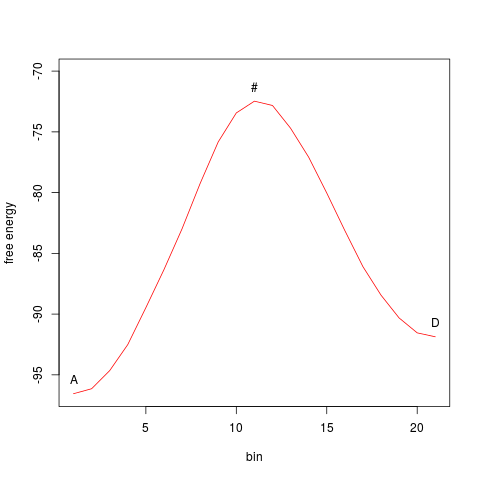
change them by Nudged Elastic BandOne of motivation of molecular modeling is identification of transition paths and transition states. In metadynminer it is possible to use Nudged Elastic Band method [3] implemented in the functionneb. First it is necessary to calculate free energy minima.
By visual inspection we can decide that it would be interesting to find a transition path between
minima A and D. The path can be analyzed by:
> tfes<-fes(acealanme)
> minima<-fesminima(tfes)
> myneb<-neb(minima, min1="A", min2="D")
> myneb
path between minima:
  letter CV1bin CV2bin       CV1      CV2 free_energy
1      A     80    235 -1.195037 2.624154    -96.5517
  letter CV1bin CV2bin       CV1       CV2 free_energy
4      D    167    152 0.9486378 0.5790386   -91.86909
> summary(myneb)
path between minima:
  letter CV1bin CV2bin       CV1      CV2 free_energy
1      A     80    235 -1.195037 2.624154    -96.5517
  letter CV1bin CV2bin       CV1       CV2 free_energy
4      D    167    152 0.9486378 0.5790386   -91.86909
with kinetics
  direction   deltag   halflife units
1        -> 24.07849   1.726768    ns
2        <- 19.39587 264.200779    ps
Minima min1 and min2 can be specified by letters or indexes.
The function Path identified by Nudged Elastic Band can be ploted:
> plot(myneb)
Alternatively, it is possible to plot it projected onto a free energy surface. This can be done
by this pair of commands (without closing the image window after the first command). The second function
works similarly to > plot(minima) > linesonfes(myneb) 
Tips and TricksPublication quality figuresFollowing script can be used to generate a publication quality figure (8x8 cm, 600 dpi):> tfes<-fes(acealanme) > png("filename.png", height=8, width=8, units='cm', res=600, pointsize=6) > plot(tfes) > dev.off()You can replace png by bmp, jpeg, tiff, pdf
or eps to get other file formates (parameters can be different).
Making FES relative to the global minimumYou can set free energy minimum to zero by typing:> tfes<-tfes-min(tfes) Hills from restarted simulationsThere are two ways to cope with hills file from restarted simulations, i.e. simulations where the time column starts from zero at every restart. It is possible to setignoretime=T in the
read.hills function. This takes the time of the first hill and use it as the uniform step.
Alternatively, it is possible to keep original times and use Making movieIndividual snapshots of a movie can be generated by:> tfes<-fes(acealanme, tmax=100) > png("snap%04d.png") > plot(acealanme, zlim=c(-200,0)) > for(i in 1:299) { + tfes<-tfes+fes(acealanme, imin=100*i+1, imax=100*(i+1)) + plot(tfes, zlim=c(-200,0)) > } > dev.off()These files can be concatenated by a movie making program such as mencoder. You can modify png functions to modify
size and resolution.
If you instead want to see flooding, type: > tfes<-fes(acealanme) > png("snap%04d.png") > plot(tfes, zlim=c(-200,0)) > for(i in 0:299) { + tfes<-tfes+ -1*fes(acealanme, imin=100*i+1, imax=100*(i+1)) + plot(tfes, zlim=c(-200,0)) > } > dev.off() Evaluation of convergence of one CVYou can use functionfes2d21d to convert a 2D surface to 1D and to evaluate
the convergence:
> tfes1<-fes2d21d(acealanme, remdim=2)
> plot(tfes1-min(tfes1), ylim=c(0,80), lwd=4, col="black")
> for(i in 1:10) {
+   tfes1<-fes2d21d(acealanme, imax=3000*i)
+   lines(tfes1-min(tfes1), col=rainbow(13)[i])
> }
Transforming CVsIf you want, for example, to use degrees instead of radians on axes, setaxes=F in the
plot function and then plot (without closing the plot window) both axes separately.
> plot(tfes, axes=FALSE)
> axis(2, at=-3:3*pi/3, labels=-3:3*60)
> axis(1, at=-3:3*pi/3, labels=-3:3*60)
> box()
The expression -3:3 will generate a vector {-3,-2,-1,0,1,2,3}, which can be
multiplied by π/3 (tick positions in radians) or by 60 (tick positions in degrees).
If you want to transform just one axis, e.g. the horizontal one, while keeping the vertical
unchanged, simply type axis(2) for the vertical one. The function box()
redraws the box.
kcal vs kJMetadynMiner works in kJ/mol by default. If your MD engine uses kcal/mol instead, you can either multiply your free energy surface by 4.184 to get kJ/mol. If you prefer to keep kcal/mol, you can seteunit="kcal/mol" for functions fes2d21d or summary
of minima and neb objects. Other units are not supported.
Shifting a periodic CVResults of some simulations with a torsion collective variable may be difficult to analyze and visualize in the range -π - +π. It may be useful to shift collective variables to 0 - 2 π. However, this problem is not very common so we did not prepare any user friendly way how to solve this. It can be solved in a user unfriendly way. Let us consider we want to shift the first collective variable to be in the range 0 - 2 π. First we will make a copy ofacealanme.
We will change its pcv1 to c(0,2*pi). Finally we can add 2 π to negative
values of the first collective variable:
> acealanmec<-acealanme
> acealanmec$pcv1<-c(0,2*pi)
> acealanmec$hillsfile[acealanmec$hillsfile[,2]<0,2]<-
+     acealanmec$hillsfile[acealanmec$hillsfile[,2]<0,2]+2*pi
> tfes<-fes(acealanmec)
> plot(tfes)
The hills file object has several instances including hillsfile, which contains the HILLS
file, and pcv1 with collective variable periodicity. They can be printed using $
operator. The expression acealanmec$hillsfile[,2] prints all values of the first collective
variable (second column). The expression acealanmec$hillsfile[,2]<0 prints the same number
of TRUE or FALSE values depending whether the first collective variable is positive or negative.
The expression acealanmec$hillsfile[acealanmec$hillsfile[,2]<0,2] prints only negative
values of the first collective variable. They can be replaced by the same value + 2 π.
References
ContactAuthor + maintenance: Vojtech Spiwok (spiwokv<you-know-what>vscht.cz)Terms of useTerms of usePrivacyPrivacy |